Meet Kou

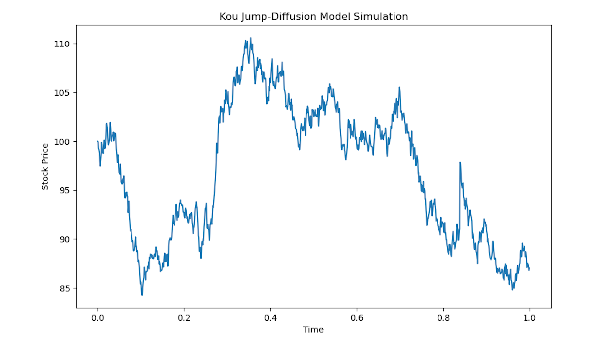
Imagine the stock price is following its usual fluctuations due to market factors (modeled by the drift and diffusion terms), but at random times, there are sudden and significant changes in price due to specific events (like earnings announcements, macroeconomic news, etc.). These events cause the stock price to “jump” discontinuously rather than change gradually.

Kou Jump-Diffusion Model

The Kou jump-diffusion model, a popular model in financial mathematics for capturing asset price dynamics with jumps. The Kou model extends the classic Black-Scholes model by incorporating double exponential jump processes to better capture the leptokurtic (i.e., heavy-tailed) and skewed nature of asset returns observed in real markets.

In the Kou model, the dynamics of the stock price \( S_t \) are given by the following stochastic differential equation (SDE):

\[ \frac{\mathrm{d} S_t}{S_t} = \mu \, \mathrm{d} t + \sigma \, \mathrm{d} W_t + \mathrm{d} \left( \sum_{i=1}^{N(t)} (J_i - 1) \right) \]

where:

• \( \frac{\mathrm{d} S_t}{S_t} \): The relative change in the stock price.
• \( \mu \): The drift term representing the expected rate of return.
• \( \sigma \): The volatility of the stock price.
• \( W_t \): A standard Wiener process (Brownian motion).
• \( N(t) \): A Poisson process with intensity \( \lambda \), representing the number of jumps up to time \( t \).
• \( J_i \): The random variable representing the relative jump size, modeled by a double exponential distribution.

Double Exponential Distribution:

The double exponential distribution used in the Kou model assumes that the log-jump sizes are distributed according to a mixture of two exponential distributions, one for positive jumps and one for negative jumps. This can be mathematically represented as:

where:

• \( Y_+ \sim \text{Exp}(\eta_1) \): The positive jump size follows an exponential distribution with parameter \( \eta_1 \).
• \( Y_- \sim \text{Exp}(\eta_2) \): The negative jump size follows an exponential distribution with parameter \( \eta_2 \).
• \( p \): The probability of a positive jump.

Complete SDE Form:

The complete SDE form of the Kou model incorporating these elements is:

\[ \frac{\mathrm{d} S_t}{S_t} = \mu \, \mathrm{d} t + \sigma \, \mathrm{d} W_t + \mathrm{d} \left( \sum_{i=1}^{N(t)} (J_i - 1) \right) \]

Interpretation:

• \( \mu \, \mathrm{d} t \): Continuous drift term.
• \( \sigma \, \mathrm{d} W_t \): Continuous diffusion term representing the random fluctuation of the asset price.
• \( \mathrm{d} \left( \sum_{i=1}^{N(t)} (J_i - 1) \right) \): Jump term representing the discontinuous jumps in the asset price.

Practical Applications:

The Kou model is particularly useful for pricing derivatives and managing risk in markets where asset prices exhibit significant jumps. It provides a more accurate reflection of market behavior compared to models that assume continuous price changes only.

Numerical Example in Python

Consider a stock with the following parameters:

• Drift (\( \mu \)) = 0.05 (5% per year)
• Volatility (\( \sigma \)) = 0.2 (20% per year)
• Poisson intensity (\( \lambda \)) = 0.1 (10% chance of jump per year)
• Positive jump parameter (\( \eta_1 \)) = 0.1
• Negative jump parameter (\( \eta_2 \)) = 0.1
• Probability of positive jump (\( p \)) = 0.5

These parameters can be used to simulate the stock price dynamics, including the impact of jumps, providing more realistic modeling of asset prices.

import numpy as np
import matplotlib.pyplot as plt

# Parameters
mu = 0.05        # drift term
sigma = 0.2      # volatility
lambda_ = 0.1    # jump intensity (rate of Poisson process)
p = 0.5          # probability of positive jump
eta1 = 0.1       # parameter for positive jump size
eta2 = 0.1       # parameter for negative jump size
T = 1            # time horizon (1 year)
n = 1000         # number of time steps

# Time increments
dt = T / n
time = np.linspace(0, T, n+1)

# Initialize stock price process
S0 = 100
S = np.zeros(n+1)
S[0] = S0

# Simulate the process
for i in range(1, n+1):
    dW = np.random.normal(0, np.sqrt(dt))
    J = 0
    if np.random.poisson(lambda_ * dt) > 0:
        if np.random.rand() < p:
            J = np.random.exponential(eta1)
        else:
            J = -np.random.exponential(eta2)
    S[i] = S[i-1] * (1 + mu * dt + sigma * dW + J)

# Plot the simulated process
plt.figure(figsize=(10, 6))
plt.plot(time, S)
plt.title('Kou Jump-Diffusion Model Simulation')
plt.xlabel('Time')
plt.ylabel('Stock Price')
plt.grid(False)

# Display the plot
plt.show()

This Python code generates the plot above, illustrating a simulated, jumpy asset price.

The Kou model is a powerful tool for financial modeling, offering both accuracy and practicality in option pricing.

The Kou model is better than the Black-Scholes model for matching historical stock prices. It’s also easier to use than other jump process models when pricing options. This is because the Kou model uses the exponential distribution, which has a special property called “memorylessness.” This property allows for explicit formulas for option prices, which makes calculations simpler and more efficient.

The Black-Scholes model assumes stock prices follow a continuous path without sudden jumps, which often doesn’t match real market behavior. In contrast, the Kou model incorporates sudden jumps in stock prices, providing a more accurate representation of actual market data. Additionally, the Kou model allows for simpler mathematical formulas to price options, making it more practical for traders and analysts. Due to the “memorylessness” of the exponential distribution, the Kou model can derive clear, straightforward formulas for pricing various options, unlike other complex jump models.

The exponential distribution has the property that the probability of an event occurring in the future is independent of the past, which allows the Kou model to handle jumps in stock prices more easily and leads to explicit pricing formulas. This provides a more realistic model of stock price movements.