In the 1960s, the Swedish actuary Gunnar Benktander found himself grappling with complex insurance claim datasets. He noticed that the prevailing Pareto and exponential distributions failed to capture nuanced patterns within the data. Driven by the need for a better solution, Benktander secluded himself in his study for an intensive weekend of work. By Monday morning, he had devised the initial version of what would become the Benktander-Gibrat distributions, poised to become a revolutionary tool for actuaries.
This groundbreaking development allowed for significantly more precise modeling of loss distributions, particularly in life insurance claims processing. Together with Jean-Marie Gibrat, Benktander aimed to create a distribution that was “intermediate” between the heavy-tailed Pareto and the light-tailed exponential, providing a flexible and accurate representation of loss data. Their innovation has since become a cornerstone in actuarial science, enhancing the industry’s ability to assess and manage risk.
The Mathematics of Benktander-Gibrat Distributions
Type I Benktander-Gibrat Distribution
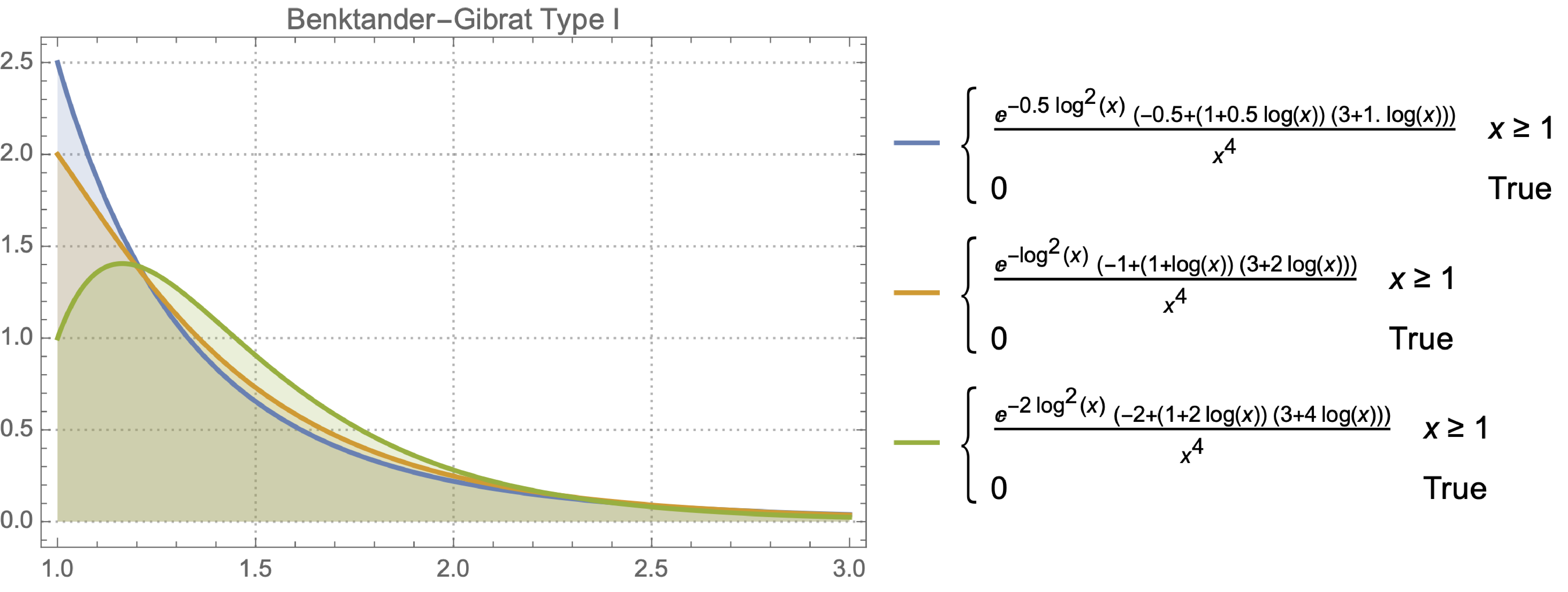
The PDF of the Type I Benktander-Gibrat distribution is given by:
\[ f(x; a, b) = x^{-a-2} \exp(-b (\log x)^2) \left((a + 2 b \log x + 1) \left(\frac{2 b \log x}{a} + 1\right) - \frac{2 b}{a}\right) \quad \text{for} \quad x > 0 \]
where \( a > 0 \) and \( b > 0 \) are shape parameters, with the restriction that \( b \leq \frac{1}{2} a (a+1) \).
The CDF is:
\[ F(x; a, b) = 1 - \exp\left(-a \log x - \frac{b}{2} (\log x)^2\right) \]

PDF of Type I Benktander-Gibrat Distribution for a range of a and b
Type II Benktander-Gibrat Distribution (also known as Benktander-Weibull Distribution)
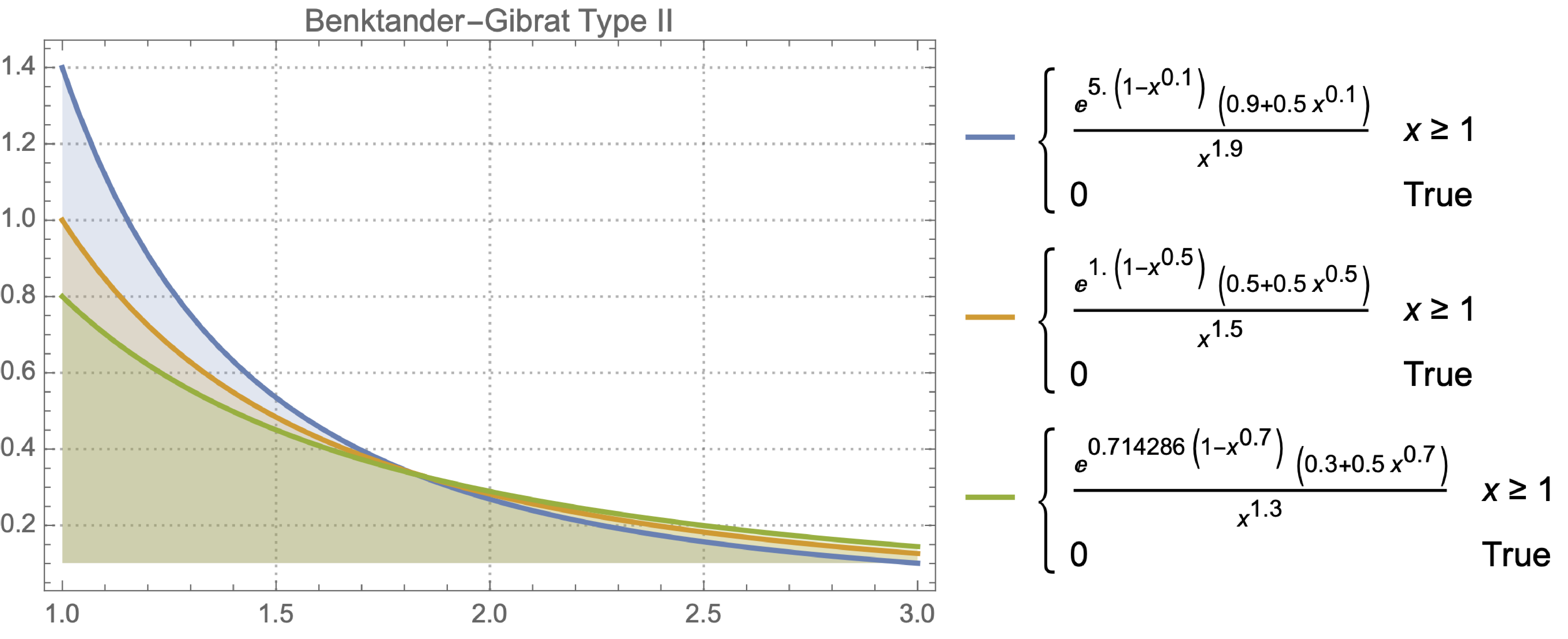
The PDF of the Type II Benktander-Gibrat distribution is given by:
\[ f(x; a, b) = (a + b \log x) x^{-1 - a} \exp(- \frac{b}{2} (\log x)^2) \quad \text{for} \quad x > 0 \]
where \( a > 0 \) and \( 0 < b \leq 1 \).
The CDF is:
\[ F(x; a, b) = 1 - x^{-a} \exp(- \frac{b}{2} (\log x)^2) \]

PDF of Type II Benktander-Gibrat Distribution for a range of a and b
Use Cases in Life Insurance Actuary Projects
-
Modeling Large Claims: Benktander-Gibrat distributions are employed to model the distribution of large life insurance claims. These distributions provide a better fit for data where the tail behavior is not as extreme as Pareto but requires more flexibility than exponential. This allows insurers to accurately estimate the probability and potential size of large claims, enhancing risk assessment and pricing strategies.
-
Risk Management and Reserving: Actuaries use Benktander-Gibrat distributions to assess risk and determine the necessary reserves for future claims. By accurately modeling the tail behavior of claim size distributions, insurers can better prepare for extreme events and ensure they have adequate reserves to cover potential losses, thereby enhancing financial stability.
-
Premium Calculation and Underwriting: The flexibility of Benktander-Gibrat distributions in capturing the nuances of claim data allows for more precise premium calculations. Underwriters can use these distributions to evaluate the risk profiles of policyholders more effectively, leading to more competitive and fair pricing of life insurance policies. This also aids in developing tailored insurance products that meet specific risk characteristics.
Suitability for Insurance Applications
-
Type I Benktander-Gibrat Distribution: This type is particularly suitable for life insurance applications due to its flexibility in modeling claim sizes and capturing the intermediate behavior between exponential and Pareto distributions. The allowance for \( a \) and \( b \) to be any real, positive numbers with \( b \leq \frac{1}{2} a (a+1) \) provides actuaries with the necessary adaptability to accurately model life insurance claim data.
-
Type II Benktander-Gibrat Distribution (Benktander-Weibull Distribution): This type is more useful for property-casualty insurance applications. Its parameters \( a \) being any positive number and \( 0 < b \leq 1 \) make it well-suited for modeling a wide range of property and casualty insurance claims, where the distribution of losses often follows patterns that can be effectively captured by the Benktander-Weibull distribution.
Understanding the Terminology
-
Benktander-Gibrat Distribution: Both Type I and Type II are often referred to under this umbrella term because they were introduced and developed by Gunnar Benktander and Jean-Marie Gibrat to model empirical mean excess functions more effectively.
-
Benktander-Weibull Distribution: Type II is specifically called the Benktander-Weibull distribution because its formulation and properties are closely related to the Weibull distribution. This naming highlights its derivation and the specific characteristics that align it with Weibull distribution properties.
Mathematical Relationship to Weibull Distribution
The Weibull distribution is widely used in reliability engineering and failure analysis. The PDF of the Weibull distribution is:
\[ f(x; k, \lambda) = \frac{k}{\lambda} \left(\frac{x}{\lambda}\right)^{k-1} \exp\left(-\left(\frac{x}{\lambda}\right)^k\right) \]
where \( k \) is the shape parameter and \( \lambda \) is the scale parameter.
The Type II Benktander-Gibrat (Benktander-Weibull) distribution can be seen as a transformation of this form, adapted to better model insurance claim data with specific properties that fall between the exponential and Pareto distributions.
Why is Type II named after Weibull?
When Gunnar Benktander and Jean-Marie Gibrat developed these distributions, they aimed to bridge the gap between the heavy-tailed Pareto and the light-tailed exponential distributions, both of which had limitations in modeling insurance claims. The Type II variant naturally aligned with certain aspects of the Weibull distribution, leading to its alternative name, the Benktander-Weibull distribution. This name helps practitioners recognize its applicability in scenarios where Weibull-like properties are desired, such as in property-casualty insurance.
By acknowledging both names, actuaries and statisticians can better understand the distribution’s derivation, properties, and suitable applications.