“In theory there is no difference between theory and practice, but in practice there is.” (Yogi Berra)
Market practitioners don’t price derivatives (such as options and futures) according to theoretical models. They take into account market conditions, supply and demand dynamics, volatility, liquidity, transaction costs, and other real-world factors that can significantly influence prices beyond theoretical assumptions.
Market practitioners who care about differences in theory and practice of derivatives pricing include:
Arbitrageurs
They exploit price discrepancies between different markets or instruments. For example, if a theoretical model suggests that an option is mispriced relative to the underlying asset, arbitrageurs will buy the underpriced option and sell the overpriced asset to lock in risk-free profits.
Market Makers
These practitioners provide liquidity by continuously quoting buy and sell prices. They benefit from the bid-ask spread and use sophisticated models to adjust their prices based on real-time market information, capturing discrepancies between theoretical values and actual market conditions.
Hedge Funds
Hedge funds often employ complex strategies to capitalize on mispricings. For instance, they might use statistical arbitrage to identify and exploit small pricing inefficiencies in a large number of derivatives simultaneously.
Prop Traders
Proprietary trading desks at banks or trading firms use their own capital to trade derivatives. They rely on advanced algorithms and real-time data to identify and profit from pricing inefficiencies that theoretical models might miss.
Institutional Investors
Large investors like pension funds and insurance companies use derivatives for hedging purposes. They benefit from understanding the practical limitations of theoretical models, allowing them to better manage risk and optimize their hedging strategies.
Retail Traders
Individual investors can also benefit from the differences between theoretical and practical pricing. By staying informed and using tools like implied volatility and market sentiment indicators, they can make more informed trading decisions.
These practitioners leverage their knowledge of market imperfections and practical constraints to enhance their trading strategies and achieve better returns.
Implied Futures Price
Suppose you want to calculated the (theoretical) futures price \(F\) of an asset, say it’s oil futures.
You look up the options data and find the following:
- Strike Price (K): $70
- Call Option Price (c): $5
- Put Option Price (p): $4.20
- Risk-Free Rate (r): 1.5% per annum (0.015)
- Time to Expiration (T): 9 months (0.75 years)
- Futures Price (F): To be calculated
Using the put-call parity formula: \[ c - p = e^{-rT} (F - K) \]
Solving for \( F \): \[ 0.8 = 0.9888 (F - 70) \] \[ F - 70 = \frac{0.8}{0.9888} \] \[ F - 70 \approx 0.809 \] \[ F \approx 70.809 \]
Practitioners call \(F\) the Implied Futures Price, I.e., the price that is derived (implied by) options data on the asset.
The implied futures price \( F \) can be derived from the relationship between call and put options on futures contracts using put-call parity.
Computing both \(F\) and \(r\) from options data
In practice, you have option price data for a futures contract. The data comes in three columns:
- \(k\) Strike price
- \(c\) Call option price
- \(p\) Put option price
You want to use this data to determine the implied futures price \(F\) and the risk-free rate \(r\), assuming all options have the same time to expiration \(T=0.5\), i.e., half a year.
Let’s get some data:
| \(k\) | \(c\) | \(p\) |
|---|---|---|
| 0.5 | 0.4907889676988285 | 0.016195946285120204 |
| 0.611 | 0.3906456841026896 | 0 |
| 0.722 | 0.26147486526332403 | 0 |
| 0.833 | 0.15317219181039937 | 0 |
| 0.944 | 0.09211854231651154 | 0.03082482601302827 |
| 1.056 | 0.032182889049210905 | 0.09805414435356587 |
| 1.167 | 0 | 0.18697027009043163 |
| 1.278 | 0 | 0.2811538815623303 |
| 1.389 | 0 | 0.3722270971672664 |
| 1.5 | 0.006944092255474923 | 0.4933152091522619 |
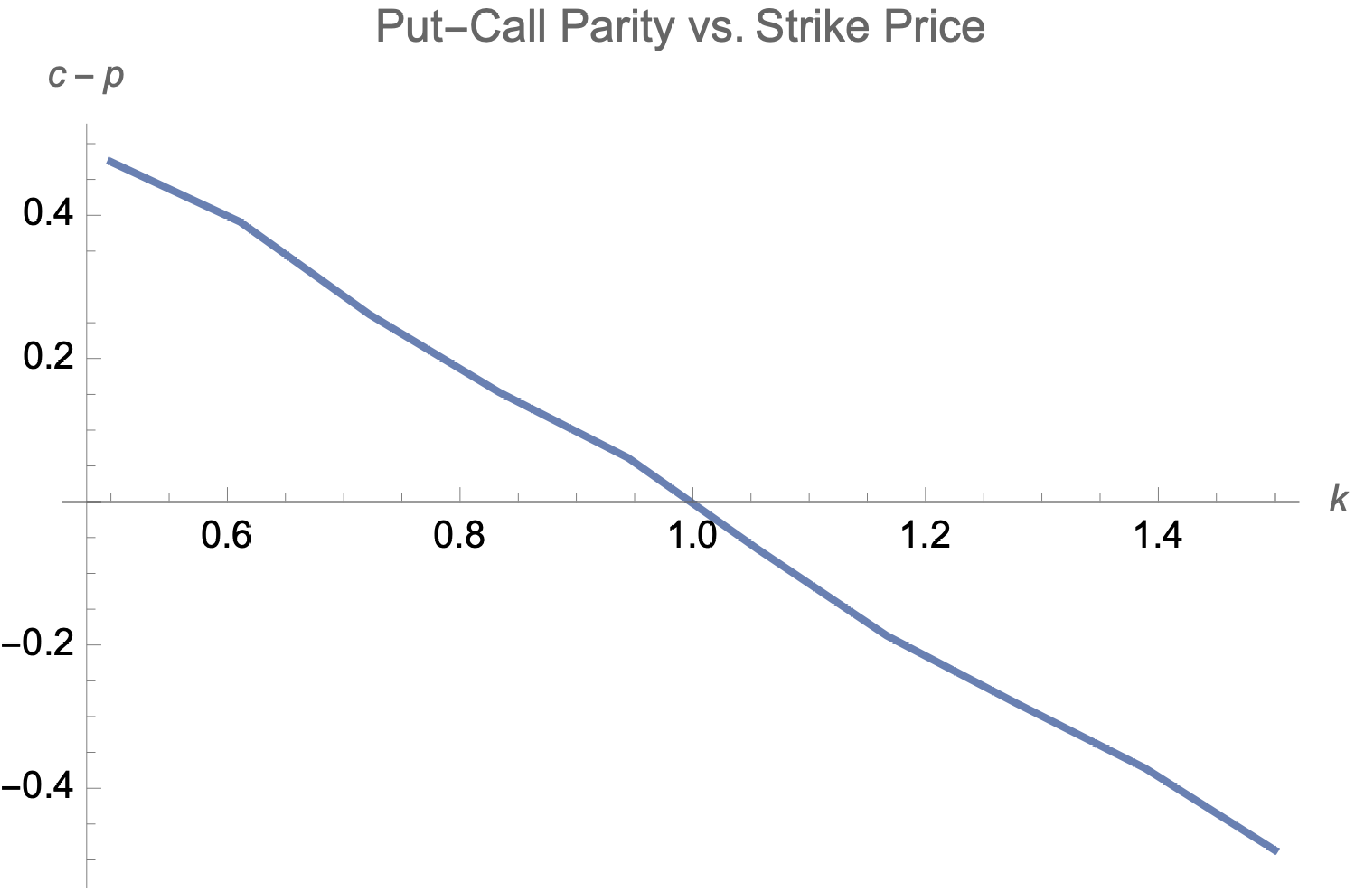
And let’s see the put-call parity \(c-p\) vs. the strike price \(k\):

Illustration of Put-Call Parity vs. Strike Price
The put-call parity formula for European options on futures is:
\[ c - p = F e^{-rT} - K e^{-rT} \]
where:
- \( c \) is the call option price,
- \( p \) is the put option price,
- \( K \) is the strike price,
- \( F \) is the futures price,
- \( r \) is the risk-free rate,
- \( T \) is the time to expiration.
Simplifying, we get:
\[ c - p = e^{-rT} (F - K) \]
From this, we can determine the implied futures price \( F \) and the risk-free rate \( r \) by using linear regression and executing the following the steps:
-
Calculate the difference between the call and put prices for each strike price: \[ c - p \]
-
Set up the equation: For each strike price \( K_i \): \[ c_i - p_i = e^{-rT} (F - K_i) \]
-
Simplify to a linear regression problem: \[ c_i - p_i = e^{-rT} \cdot F - e^{-rT} \cdot K_i \]
-
Rewrite it as: \[ c_i - p_i = A \cdot F - A \cdot K_i \] where \( A = e^{-rT} \).
You can now use Python (or Mathematica, or R) to perform linear regression to estimate the slope \( A \) (which is \( e^{-rT} \)) and the intercept divided by \(A\), i.e., the implied futures price \( F \).
You should get \(F = \$0.994719\) and \(r = 0.0534882\).